A Gentle Introduction to Computational Quantum Mechanics

On mobile devices, read the page in horizontal/"landscape" mode. Otherwise math may not fit the screen.

This little text is intended as a very simple introduction to computational quantum mechanics. There are many books devoted to the topic, filled with one complicated algorithm after the other. Many people devote their whole careers to computational quantum mechanics. It’s harder to find something that allows a total beginner to get started.

Unfortunate, isn’t it? After all, you don’t teach a fella how to drive by putting him in a Formula 1 car; you don’t teach a soldier to fire a weapon by placing him in front line combat; you can’t teach a child to run a marathon when she has yet to take her first steps.

Fortunately, it’s not too difficult to write programs that solve the quantum equations on a computer. In fact, we can solve the problem and plot the solution in just a few lines of Python code. To understand those lines, though, takes a little bit of work. It’s easy to see a painting and say "well, just take a brush and move it around the paper a bit!" It’s a bit harder to do that in practice. In the cases we’ll solve, though, it’s not that difficult. All I require of the reader is the basics of linear algebra, calculus and some programming knowledge, that’s all; the linear algebra and calculus are a bare minimum for quantum mechanics, and programming should go without saying since we’re doing computational work!

Hopefully the reader doesn’t already feel betrayed — I did say I wouldn’t teach a kid to run a marathon before they can walk. In this case, though, knowing some calculus and linear algebra is the equivalent of standing up. If you haven’t yet heard of those, you have two options: don’t read further or just blindly copy the code to see the end results to get yourself motivated to learn calculus.

I will program in Python, so to follow along, make sure you have numpy and matplotlib installed. Then write these at the top of your file:

import numpy as np
import matplotlib.pyplot as plt

We’re ready to go! We’ll solve the time-independent Schrödinger equation in one dimension

\[\begin{aligned} \bigg( -\frac{1}{2} \frac{d^2}{dx^2} + V(x)\bigg)\psi (x) = E\psi (x)\end{aligned}\]

If you’ve taken quantum mechanics, you might have heard that this is an eigenvalue equation, and that’s one of the reasons Schrödinger’s equation produces "quantization" (discrete energy levels with allowed values some distance apart). But if you know a bit of linear algebra, you know that eigenvalues are something matrices have. So what the hell do I mean, eigenvalues? That’s not a matrix on the left hand side!

What Do You Mean, Eigenvalues?

The bad news is that the theory of "eigenvalues" of operators such as $-\frac{1}{2}\frac{d^2}{dx^2}$ is pretty complicated. The good news is that we don’t need it, because we can approximate this operator as a matrix.

I can hear you huffing and puffing in indignation. How on earth could a derivative be a matrix?

Calm yourself, all will be revealed. Let’s think about what we need to fit the equation on a computer.

First of all, we don’t have an infinite amount of memory. Unfortunately, $\psi (x)$ contains an infinite number of points. That’s not some special magic of the wave function, it’s true for any function defined on real numbers – like $f(x) = x^2$. Since there’s an infinite number of real numbers in any interval, the function is also defined on an infinite number of points.

Too bad we don’t have an infinite amount of memory to store this infinity of numbers. We have to store just a finite number instead. Can you think of any way to do so?

One way – the one we’ll follow – is to just divide some finite interval in to a number of smaller bits, and define just one number as the value of the function in these bits.

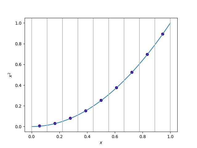
Confused? Not to worry, here’s what I mean. Let’s suppose we want to write the function $f(x) = x^2$ in the interval [0,1]. We might divide this in to a number of smaller intervals:

\[\begin{aligned} = [0,0.1]\cup [0.1,0.2]\cup \dots \end{aligned}\]

Then we say, the value in the first small interval is, for example, the average value of the function at the starting point and end point. So, in the first interval, it’s $\frac{f(0)+f(0.1)}{2} = \frac{0^2 + 0.1^2}{2} = 0.005$, and so on. These values then form the discrete version of the function.

What does this have to do with our Schrödinger equation? Well, look at the derivative on the left hand side – we have to define it on a finite set of points instead of a continuous function. Let’s recall the definition of a derivative:

\[\begin{aligned} \frac{df}{dx} = \lim _{h\rightarrow 0}\frac{f(x+h)-f(x)}{h}.\end{aligned}\]

We now replace the limit $h\rightarrow 0$ with the limit $h\rightarrow \Delta x$, with $\Delta x$ the length of the small intervals. For instance, the derivative at the first interval of $x^2$ would be

\[\begin{aligned} \frac{f(0.1)-f(0)}{0.1} = \frac{0.1^2-0^2}{0.1} = 0.1\end{aligned}\]

Let’s see what this looks like graphically. If you want to generate these plots yourself, it’s actually simple: we can create evenly spaced values using numpy and then use matplotlib to get the figures. Like so:

import numpy as np
import matplotlib.pyplot as plt

xcont = np.linspace(0,1,100000) # "Continuous" x
x = np.linspace(0,1,10) # Discrete approximation

xsqdisc = [] 
for i in range(len(x)-1): # Filling the array with the approximation
    xsqdisc.append((x[i+1]**2+x[i]**2)/2) # outlined in the text

plt.xlabel("$x$")
plt.ylabel("$x^2$")
plt.scatter(x[:len(x)-1]+(x[1]-x[0])/2,xsqdisc, color="indigo")
plt.plot(xcont,xcont**2)
for i in x: # This creates the silvery vertical lines
    plt.axvline(x=i, color = "silver")

plt.show()

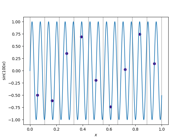
You see that the dots land pretty nicely on the line; perhaps this is a good approximation to our function! Beware, though – if the function changes too much within the span of one interval, then we might get a very poor approximation if our intervals are too large. For example, look at this approximation of a rapidly oscillating $\sin (x)$:

Not very good, is it? The function oscillates too much between each interval, so our approximation is way off. Obviously, trying to compute the derivative using this approximation would be especially useless, since it would miss all the detail in between each interval! By the way, you should try to generate that picture yourself as well, as practice.

So, the key thing is to have a sufficient number of points to guarantee a good approximation. More points = better, typically.

What bearing does this have on our Schrödinger equation? Well, every school boy can now guess that if we represent the wave function as a set of points:

\[\begin{aligned} \psi (x) \approx \begin{bmatrix} \psi (x_1)\\ \psi (x_2)\\ \psi (x_3)\\ \vdots \end{bmatrix}\end{aligned}\]

then the discrete approximation of the Hamiltonian must be a finite-dimensional matrix. So it’s just a normal eigenvalue problem after all, and it makes a whole lot of sense to talk about eigenvalues.

About That Derivative

Well, then, what matrix is it? Remember how we defined the derivative on finite intervals:

\[\begin{aligned} \frac{df}{dx} = \frac{f(x+\Delta x) - f(x)}{\Delta x}\end{aligned}\]

The second derivative approximation (well, one of them) is

\[\begin{aligned} \frac{d^2f}{dx^2} = \frac{f(x+\Delta x)+f(x-\Delta x)-2f(x)}{(\Delta x)^2}\end{aligned}\]

(Can you derive this? Use the backward-difference definition for the derivative on the first derivative!)

So how do we find a matrix, say $D$, the effect of which is:

\[\begin{aligned} D\begin{bmatrix} \vdots\\ \psi (x_i)\\ \vdots \end{bmatrix} =\frac{1}{(\Delta x)^2} \begin{bmatrix} \vdots\\ \psi (x_{i+1}) + \psi(x_{i-1}) - 2\psi (x_i)\\ \vdots \end{bmatrix}\end{aligned}\]

At first, this might seem like a daunting task, since we don’t even know how big our matrix needs to be. Luckily, there’s a simple pattern here which we can exploit. We can easily discover it by writing the matrix multiplication by components. If our $\psi$ has $N$ points, then the $i$th element of the multiplication is

\[\begin{aligned} (D\vec{\psi})_i = \sum _{j=1}^N D_{ij}\psi _j\end{aligned}\]

where the $D_{ij}$ indicates the elements in $i$th row and $j$th column. Convince yourself that this is indeed the matrix multiplication rule you learned in linear algebra, if you don’t see it immediately! Try it with something simple, like a 2-by-2 matrix and a 2-dimensional vector.

Well, we know what we want on the right hand side. When $j = i$, we want the coefficient $-2$, so $D_{ii} = -2$. When $j=i\pm 1$, we want the coefficient $D_{i(i\pm 1)} = 1$. The rest of them must be zero. Then:

\[\begin{aligned} \sum _{j=1}^N D_{ij}\psi _j &= D_{ii}\psi _i + D_{i(i+1)}\psi _{i+1} + D_{i(i-1)}\psi _{i-1}\\ &= \psi (x_{i+1}) + \psi(x_{i-1}) - 2\psi (x_i)\end{aligned}\]

Then we just need to multiply by $1/(\Delta x) ^2$, which is just a constant. So we end up with the matrix:

\[\begin{aligned} D = \frac{1}{(\Delta x)^2} \begin{bmatrix} -2 & 1 & 0 & \cdots \\ 1 & -2 & 1 & \ddots \\ 0 & 1 & -2 & \ddots \\ \vdots & \ddots & \ddots & \ddots \end{bmatrix}\end{aligned}\]

The three central diagonals are non-zero, everything else is zero. Now remember that in the Hamiltonian, we also have the factor $-\frac{1}{2}$, so we have to multiply that in as well.

Let’s build this matrix in Python. Once again, numpy to the rescue. There’s a function called diagflat that allows us to easily make matrices from vectors. The second argument indicates how many diagonals above the central diagonal we want to put our vector. Those are smaller than the central diagonal, so we need smaller arrays of coefficients. Like so:

import numpy as np
import matplotlib.pyplot as plt
x = np.linspace(0,1,1000)
dx = x[1]-x[0]
N = len(x)

D2 = -0.5/dx/dx * (np.diagflat(-2 * np.ones(N)) \
+ np.diagflat(np.ones(N-1), -1) + np.diagflat(np.ones(N-1),1))

Let’s take a step back for a moment. If you’ve ever solved the Schrödinger equation, you know that you need boundary conditions. Without them, solving it is like wandering around in an unknown city with no map – you’re going to wake up in a ditch with a hell of a hangover. Or something.

Well, we’ve just constructed a matrix, so what are the boundary conditions on the $\psi$ given by it? Do the multiplications to examine the first and last element of the $\psi$-vector after multiplication:

\[\begin{aligned} \psi = \begin{bmatrix} \psi _{x_2} - 2\psi _{x_1}\\ \vdots \\ \psi _{N-1} - 2\psi _{x_N} \end{bmatrix}\end{aligned}\]

See something funny? Only two terms. That’s because our matrix sort of "cuts off" at the edges. What does this mean? Well, evidently $\psi_{x_0}$ vanishes from the equation, so it must be 0! We’re so clever that we’ve taken care of the boundary conditions without even trying. Three cheers for us!

Basically, then, this system should depict a particle in a box - a favorite model of physics teachers everywhere. And fortunately, this system can be solved analytically. The eigenenergies are

\[\begin{aligned} E_n = \frac{\pi ^2n^2}{2L^2}\end{aligned}\]

For simplicity, why not make our box length $L=1$?

To recap, taking the matrix we called D2 in Python, we should get as the first eigenvalue $\pi ^2/2$, the second eigenvalue $\pi ^2\cdot 4 /2$, and so on. Well, let’s solve them then. Luckily numpy makes this easy for us. Add this to your code:

e,vec = np.linalg.eigh(D2)
plt.scatter([1,2,3,4],e[:5])
plt.scatter([1,2,3,4], [np.pi**2/2,\ 
 4*np.pi**2/2, 9*np.pi**2/2, 16*np.pi**2/2])
plt.show()

You should see them match very well. But you’ll notice that the higher eigenvalues are off by larger margin. Why?

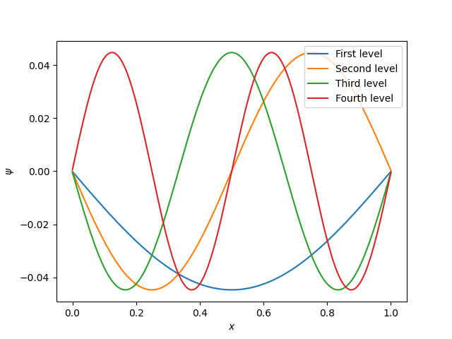
The higher the energy, the more wiggly the wave function is. To see this, you can plot the wave functions; they’re now stored in the variable vec so that vec[:,0] is the first eigenvector, vec[:,1] the second and so on. But the more wiggly the wave function, the worse our division in to intervals is likely to be, as we saw before withou our $\sin (x)$ example. So the derivative matrix is going to be a worse approximation!

Don’t believe me? Here’s the first few wave functions:

See? More wiggly. More change over one interval. Worse approximation.

But What About The Potential?

Ah, but we haven’t dealt with the pesky $V(x)$ yet! Is it because it’s too difficult? No – I’ve left it for last so that you can have an easy finish. It’s like taking an exam, you don’t want to do the toughest problem last, when you’re already exhausted. (Incidentally, I almost always did that, anxious to at least get the easy stuff out of the way. Then I couldn’t focus on the hard ones. Oh well..)

What’s the effect of a potential depending on $x$ on $\psi (x)$? Well, you just multiply $\psi (x)$ at each point $x$. So in matrix terms,

\[\begin{aligned} \hat{V}\vec{\psi} = \begin{bmatrix} \vdots \\ V(x_i)\psi (x_i)\\ \cdots \end{bmatrix}.\end{aligned}\]

A moment’s thought shows that this must be a diagonal matrix. So, for example, the harmonic oscillator potential is as simple as:

xsq = np.diagflat(x**2)

The total Hamiltonian is then the sum D2+xsq. Make sure this gives the correct eigenvalues for a harmonic oscillator, too!

Recap, conclusions, where to from here?

So there we go, this computational QM stuff isn’t so hard after all. Declare yourself the master – nay, the PhD of – nay, the PROFESSOR of computational quantum mechanics, right?

Well, not quite. The method we’ve applied here is very naive and not reliable or workable for complicated systems. Unfortunately the number of points needed tends to sort of explode in 3 dimensions. This method is not really used by the professionals.

What is done instead is that you guess the form of the wave function. Instead of writing $\psi$ on a finite set of points, you expand it in terms of some known functions:

\[\begin{aligned} \psi (x) = \sum _i^{N} c_i \phi _i(x).\end{aligned}\]

We choose $\phi _i$ in a clever way so that they’re already pretty close to the solution. Doing this is as much art as it is science, but even a relatively bad guess of this form leads to a numerically much easier problem and thus better results. That’s for another time, though.

You should use the code we have to explore random potentials you find interesting. Send me email if you see something funny. I like funny things.