Scaling in the Ising Model
On mobile devices, read the page in horizontal/"landscape" mode. Otherwise math may not fit the screen.This is a first introduction to numerical renormalization methods. In terms of the code, I followed the tutorial in1.
Basics of the Ising Model
The Ising model is a well-studied and simple theory for magnetization. The basic idea of the model is to consider a grid (in our case, either 1D chain or 2D grid) of spins, some of which "point up" (and thus have value +1) and some of which "point down" (have value -1). The energy of the system is then
\[\begin{align} E = -J\sum _{\langle ij\rangle} s_is_j \label{eq:energyising}\end{align}\]with $\langle ij\rangle$ indicating nearest-neighbor sums. So, it is a very simple thing to compute: just go over each of the spins, and take products with its (non-diagonal) neighbors.
The code used for the graph in this text is just a basic Ising Monte Carlo code; since the model is a staple of physics teachers everywhere, it is easy to find tutorials on how to make your own. I won’t spend time on it in this article.
Scaling
The basic question of scaling (renormalization) methods is this: what happens if you zoom out of the system?
By zooming out, I mean the following. Take a grid containing, say, $9\cdot 9$ cells, with some arrangement of spins. What if we treated this grid in some averaged fashion to save some work?
This question pops up quite frequently in physics. In particle physics, things like masses of particles going in to the equations are different depending on what energy scale you’re looking at. Calculations with "bare" masses tend to produce infinite results that have to be removed by basically inserting some energy-dependence.
Obviously, the dependence of our quantity of interest on $J$ in $\eqref{eq:energyising}$ doesn’t have to stay the same in this "zooming out" process. We must work out some way to find a function, say $R(J)$, which takes in a coupling constant and returns the coupling constant for a coarser model which keeps the magnetization unchanged.
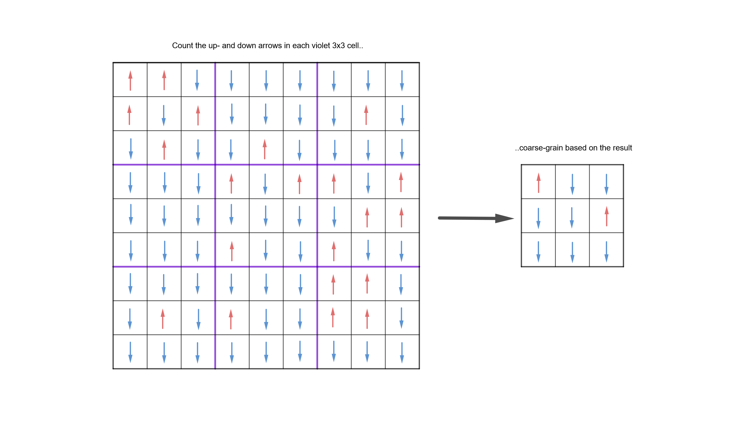
How could we find this function? Well, first we must get the magnetization for the large grid, $9 \cdot 9$. Then we average over this grid somehow. For example, we could divide it in to blocks of size $3\cdot 3$, and have the spins in those blocks "vote": if there are more up-spins than down-spins, the averaged block has an up spin, and vice versa. We now compute this "coarse-grained" (CG) magnetization. Then, we compare it to a native 3x3 grid, one where we didn’t average over the cells, but rather just did the calculation in the 3x3 system straight away. Here’s a picture of coarse graining:

To recap, at this point we have two functions: $ \langle M_{3\cdot 3}(J)^2 \rangle $ and $ \langle M_{3\cdot 3}^{CG }(J)^2\rangle $. But these two are not necessarily the same: coarse-grained magnetization probably doesn’t match the native 3x3 calculation.
If we want to see how to change J to get the same results in both methods, we have to find a function such that:
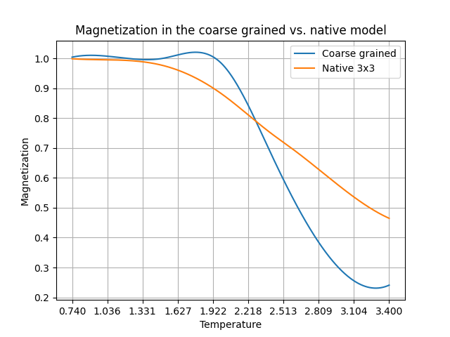
\[\begin{aligned} \langle (M_{9\cdot 9}^{CG }(J))^2\rangle = \langle M_{9\cdot 9}^2(J')\rangle, \quad J'=R(J)\end{aligned}\]So the sensible thing to do is to plot these two curves in the same plot, and try to work out the function $R(J)$ from there. We can see what the function is just visually by looking at the picture:

We can see that in the picture above.
What is the meaning of the point at which the lines cross? At those points, evidently, the coupling constants are same at both scales for the same magnetization. Remember that the calculation only depends on $\beta J=J/T$, not $\beta$ and $J$ separately; changing one is equivalent to changing the other. So at approximately the point $T = 2.3$, it doesn’t matter at which scale we look at the problem, coarse grained or not.
One of Ken Wilson’s great triumphs was understanding that these fixed points denote phase changes. In fact, a characteristic property of phase changes is that they depend on all scales. When the magnet is changing from a ferromagnet to non-magnetic, it is not merely a local, small-scale phenomenon, nor is it merely a large-scale aggregate issue. When the phase change happens, it happens at every scale simultaneously; all scales, both long-range and short-range, high-energy and low-energy, contribute to the system. It is precisely this property that makes phase change so dramatic.
The relationship of this to renormalization in QFT is that it’s basically the same process. The masses and coupling constants depend on the scale. The method I’ve used in this post is just an extremely clumsy and bad way to figure out how things change at scale and where the phase transitions are, but there are better ones. I will look at one of them in the Part 2 of this series (stay tuned..).